
Excel is a popular spreadsheet software developed by Microsoft that allows users to create, manipulate, and analyse data in various formats, including graphs. Excel graphs, also known as charts, are visual representations of data that provide insights and help users understand data patterns, trends, and relationships more easily.
Excel provides a wide range of graph types, such as line charts, bar charts, pie charts, scatter plots, and more, which can be created from data entered into the spreadsheet or imported from external sources. Excel graphs can be customised with various formatting options, including colours, fonts, titles, labels, legends, and axes, to create visually appealing and informative representations of data.
Excel graphs are useful for a wide range of applications, including business, finance, science, engineering, education, and more. They can be used to display data trends over time, compare data sets, highlight patterns, identify outliers, and communicate information effectively to stakeholders or decision-makers.
Creating Excel graphs involves selecting the data to be plotted, choosing the appropriate graph type, and customising the graph settings to suit the specific data and visualisation requirements. Excel graphs can be updated dynamically as data changes, making them a powerful tool for data analysis and reporting.
In summary, Excel graphs are a powerful feature of Microsoft Excel that enable users to create visually appealing and informative representations of data, helping them analyse and communicate data patterns and trends effectively.
How to do a graph with Excel?

Sure! Creating a graph in Excel involves several steps. Here’s a detailed guide on how to create a basic graph using Excel:
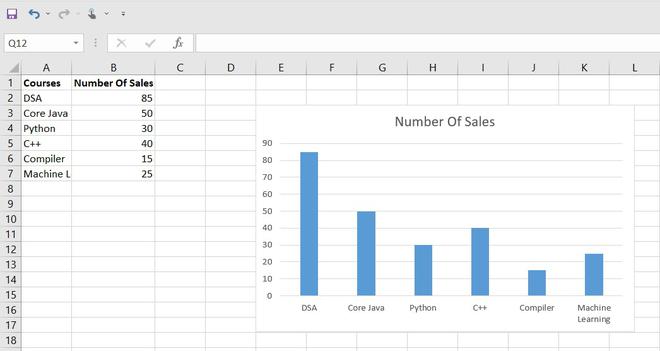
Step 1: Enter Data in Excel
Enter the data that you want to plot on a graph into an Excel spreadsheet. The data should be organised in columns or rows, with labels in the first row or column to identify each data set.
Step 2: Select Data for the Graph
You can include any data in the graph you wish.You can include any data in the graph you wish. You can do this by clicking and dragging over the data cells with the mouse or by using the Ctrl key and selecting individual cells or ranges of cells. Make sure to include any labels or headers that you want to be displayed on the graph.
Step 3: Choose Graph Type
Once you have selected the data, go to the “Insert” tab in the Excel toolbar and click on the “Recommended Charts” or “Charts” button. This will open the “Insert Chart” window where you can choose from various graph types, such as line chart, bar chart, pie chart, scatter plot, and more. You can also preview the chart types to see how they will look with your data.
Step 4: Customise Graph
After selecting a graph type, Excel will automatically generate a basic graph using the selected data. You can then customise the graph by right-clicking on different elements of the graph, such as the title, axis labels, data series, and legend, and choosing the formatting options from the context menu that appears. You can also use the “Chart Elements” button on the toolbar to add or remove specific elements from the graph.
Step 5: Update Graph with Data Changes
If you need to update the graph with changes in the data, simply modify the data in the spreadsheet, and the graph will update automatically. You can also right-click on the graph and choose the “Select Data” option to modify the data series or add/remove data.
Step 6: Save and Share Graph
Once you have customised the graph to your satisfaction, you can save the Excel file, including the graph, by clicking on the “File” tab and selecting “Save As.” You can choose the desired file format, such as .xlsx, .csv, or .pdf, and specify the save location. You can also copy and paste the graph into other applications, such as Word or PowerPoint, or directly share it with others by using Excel’s sharing options.
That’s it! You have now created a graph in Excel. You can further explore Excel’s extensive chart formatting options and features to create more complex and visually appealing graphs to suit your specific needs.
What is the formula for series in Excel?
In Excel, the formula for creating a series is a sequence of values that follow a pattern or increment by a constant value. Excel provides several built-in functions that can be used to generate a series of numbers or other types of data. Here are some commonly used formulas for creating series in Excel:
The “SERIES” Formula:
- The “SERIES” formula is used to generate a series of values based on a specified pattern or formula. The syntax for the “SERIES” formula is as follows:
SERIES(name, categories, values, plot_order, plot_by)
where:
- “name” is the name of the data series, which will be displayed as the legend in the chart.
- “categories” is the range of cells that define the categories (X-axis) for the series.
- “values” is the range of cells that define the values (Y-axis) for the series.
- “plot_order” is an optional argument that specifies the order in which the series should be plotted on the chart.
- “plot_by” is an optional argument that specifies whether the series should be plotted by rows or columns.
The “ROW” and “COLUMN” Formulas:
- The “ROW” and “COLUMN” formulas are used to generate a series of numbers in a single column or row, respectively. Here is the syntax: Here is the syntax:
ROW(start_value,[step]) =COLUMN(start_value,[step])
where:
- “start_value” is the first value in the series.
- “step” is an optional argument that specifies the increment value for each subsequent number in the series.By default, 1 is used if not specified.
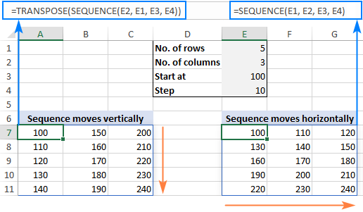
The “SEQUENCE” Formula:
- The “SEQUENCE” formula is available in Excel 365 and later versions and is used to generate a sequence of numbers or dates in a single column or row. The syntax for the “SEQUENCE” formula is as follows:
SEQUENCE(rows,[columns],[start],[step])
where:
- “rows” is the number of rows in the generated sequence.
- “columns” is an optional argument that specifies the number of columns in the generated sequence. A value of ,1 is the default if no value is specified, which generates a single column.
- “start” is an optional argument that specifies the starting value of the sequence. A default value of 1 is used if not specified.
- “step” is an optional argument that specifies the increment value for each subsequent number in the sequence. If not specified, the default value is 1.
These are just some of the formulas that can be used to generate series in Excel. Depending on your specific requirements and data patterns, you may need to use other formulas or combinations of formulas to create the desired series of data. Excel offers a wide range of formulas and functions that can be combined in various ways to generate and manipulate data for charts, calculations, and other purposes.
Types of graphs in excel
Excel offers a wide range of graph types that can be used to visualise data in various formats. Here are some of the commonly used graph types in Excel, along with a brief description of their features and use cases:
- Column Chart: A column chart displays data in vertical columns, where the height of each column represents the value of a particular data point. Column charts are used to compare data across different categories or to track changes in data over time.
- Bar Chart: A bar chart displays data in horizontal bars, where the length of each bar represents the value of a particular data point. Bar charts are used to compare data across different categories, similar to column charts, but with a horizontal orientation.
- Line Chart: A line chart displays data as a series of points connected by lines, which represent the trend or change in data over time. Line charts are used to show trends, patterns, or changes in data over continuous intervals, such as time series data.
- Pie Chart: A pie chart displays data as a circle divided into slices, where the size of each slice represents the proportion or percentage of a particular data point in relation to the total. Pie charts are used to show proportions or percentages of data in a whole or to compare data across different categories as parts of a whole.
- Scatter Plot: A scatter plot displays data as individual points plotted on a graph, where the position of each point represents the values of two different data points on the X and Y axes. Scatter plots are used to show the relationship or correlation between two sets of data points and identify patterns or trends.
- Area Chart: An area chart displays data as a series of points connected by lines and filled areas, which represent the cumulative or total value of data over time. Area charts are used to show the trend or change in data over time, similar to line charts, but with the area under the line filled with color.
- Bar and Column Combined Chart: This type of chart combines both bar and column charts in a single graph, allowing for easy comparison of data across categories and different data types, such as quantities and percentages.
- Other Chart Types: Excel also offers other chart types such as scatter with straight lines, scatter with smoothed lines, bubble chart, radar chart, stock chart, and more, which are useful for specific data visualisation requirements.
These are some of the commonly used graph types in Excel, but the list is not exhaustive. Excel provides a wide range of chart types and customization options to suit different data visualisation needs. The choice of the appropriate graph type depends on the type of data, the message you want to convey, and the insights you want to highlight from the data.
The best way to graph large amounts of data in Excel
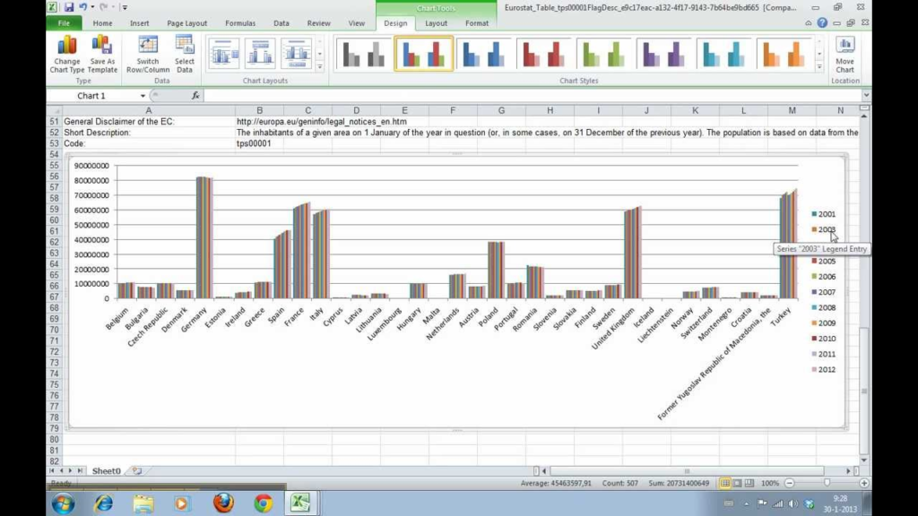
Step 1: Prepare Your Data
Make sure your data is organized in a tabular format with the data you want to graph in columns or rows. Ensure that you have meaningful column or row labels to represent the data accurately.
Step 2: Select Data
Highlight the range of data that you want to include in your graph. You can do this by clicking and dragging your mouse over the cells containing the data, or by using keyboard shortcuts such as Ctrl + Shift + Right Arrow to select an entire row or Ctrl + Shift + Down Arrow to select an entire column.
Step 3: Choose Chart Type
Go to the “Insert” tab in the Excel toolbar and click on the “Recommended Charts” or “Charts” button. Excel will automatically suggest chart types based on the selected data. Alternatively, you can manually select a chart type from the “Charts” section in the toolbar.
Step 4: Customise Chart
Once you have selected a chart type, Excel will insert a chart into your worksheet. You can now customize the chart by right-clicking on various elements of the chart, such as data points, axes, and titles, to access formatting options. You can also use the “Chart Elements” and “Chart Styles” buttons in the Excel toolbar to further customize your chart.
Step 5: Add Data Labels
If your data set is large, you may want to add data labels to your chart to help interpret the data. You can do this by right-clicking on the data points in the chart and selecting “Add Data Labels” from the context menu. Data labels can display the actual values or other data point properties such as labels or percentages.
Step 6: Format Data Axis
If your chart includes an axis, you can format it by right-clicking on the axis and selecting “Format Axis” from the context menu. This allows you to customize the axis scale, tick marks, labels, and other properties to suit your needs.
Step 7: Save and Share
Once you have created and customized your chart, you can save your Excel file to retain your graph. You can also copy and paste your chart into other applications such as Word or PowerPoint, or export it as an image or PDF for sharing or printing.
These are the general steps to create a Excel graph with a large amount of data. Excel provides extensive customization options, allowing you to create visually appealing and informative graphs to effectively convey insights from your data.
Excel graph templates
Excel graph templates are pre-designed graph layouts that you can use as a starting point to create professional-looking graphs in Excel quickly and easily. These templates are designed to save you time and effort by providing pre-set formatting, styles, and layouts that can be customized to suit your specific data and presentation needs.
Here are some further details about Excel graph templates:
- Built-in Excel Templates: Excel comes with a variety of built-in graph templates that you can access through the “Insert” tab in the Excel toolbar. These templates cover a wide range of chart types, including bar charts, line charts, pie charts, scatter plots, and more. You can choose a template that closely matches the type of graph you want to create, and then customize it with your own data and formatting.
- Online Templates: Excel also allows you to access a collection of online templates, which are created and shared by other Excel users or Microsoft. You can access these templates from within Excel or by visiting the Microsoft Office website. These templates provide a wider range of options and styles, and you can search for templates based on specific industries, purposes, or themes.
- Customising Templates: Once you select a graph template, you can customize it to suit your specific needs. You can modify the chart title, data labels, legend, axis labels, colors, fonts, and other formatting options to match your data and presentation requirements. You can also add or remove chart elements, such as data points, trendlines, or annotations, to further enhance your graph.
- Saving and Reusing Templates: After you have customized a graph template, you can save it as your own custom template for future use. This allows you to create consistent and professional-looking graphs across different presentations or worksheets. To save a graph as a template, simply right-click on the graph and select “Save as Template” from the context menu. You can then access your custom templates from the “Templates” section in the Excel toolbar.
- Creating Your Own Templates: If you frequently use a specific graph format or style that is not available in the built-in or online templates, you can create your own graph templates from scratch. Simply customize a graph to your liking, and then save it as a template for future use. You can also share your custom templates with others or download templates created by others for your own use.
Excel graph templates are a useful tool for creating visually appealing and professional-looking graphs in Excel. They provide a starting point for creating charts that are visually appealing, informative, and customized to your specific data and presentation needs.
Faqs
Here are some frequently asked questions (FAQs) about Excel graphs, along with brief answers:
Q1. How do I create a graph in Excel?
To create a graph in Excel, you can follow these steps:
a. Select the data you want to plot in the graph.
b. Go to the “Insert” tab in the Excel toolbar.
c. Choose the desired graph type from the “Charts” section, such as bar chart, line chart, pie chart, etc.
d. Excel will insert the selected graph into your worksheet, and you can customize it further as needed.
Q2.How do I customize the appearance of a graph in Excel?
You can customize the appearance of a graph in Excel by right-clicking on various elements of the graph, such as data points, axes, titles, and legends, and selecting formatting options from the context menu. You can also use the “Chart Tools” tab in the Excel toolbar to access additional formatting options, such as changing colors, fonts, styles, and more.
Q3.How do I add data to an existing graph in Excel?
To add data to an existing graph in Excel, you can follow these steps:
a. Select the graph by clicking on it.
b. Excel’s toolbar has a tab called “Chart Tools”.
c. In the “Data” group, click on “Select Data.”.
d. Click on the “Add” button in the “Legend Entries (Series)” box.
e. Enter the new data range and series name in the “Edit Series” dialog box.
f. Click “OK” to add the new data to the graph.
Q4.How do I change the type of graph in Excel?
To change the type of graph in Excel, you can follow these steps:
a. Select the graph by clicking on it.
b. Excel’s toolbar includes a tab called “Chart Tools.”.
c. Click on the “Change Chart Type” button in the “Type” group.
d. Choose the desired graph type from the list of available options.
e. Excel will automatically update the graph to the new type.
Q5.How do I create a combination graph with multiple data sets in Excel?
To create a combination graph with multiple data sets in Excel, you can follow these steps:
a. Select the data you want to plot in the graph, including all the data sets.
b. Go to the “Insert” tab in the Excel toolbar.
c. Choose a graph type that supports multiple data sets, such as a line chart or scatter plot.
d. Excel will insert the selected graph type into your worksheet with multiple data sets.
e. You can then customize the appearance and formatting of the graph as needed.
Q6.How do I add trendlines or data labels to a graph in Excel?
To add trendlines or data labels to a graph in Excel, you can follow these steps:
a. Select the graph by clicking on it.
b. Excel’s toolbar has a “Chart Tools” tab.
c. Click on the “Add Chart Element” button in the “Chart Elements” group.
d. Choose the desired chart element, such as trendline or data labels, from the list of available options.
e. Excel will add the selected chart element to the graph, and you can customize it further using the formatting options available.
Q7.How do I save a graph as an image or PDF in Excel?
To save a graph as an image or PDF in Excel, you can follow these steps:
a. Select the graph by clicking on it.
b. Right-click on the graph and choose “Save as Picture” or “Save as PDF” from the context menu.
c. Choose the desired location and file format for the saved image or PDF.
d. Click “
Conclusion
In conclusion, Excel provides a powerful and flexible tool for creating various types of graphs and visualisations to represent data in a visually appealing and meaningful way. With Excel’s charting capabilities, you can easily create and customise different types of graphs, such as bar charts, line charts, pie charts, scatter plots, and more, to effectively display your data. You can also customize the appearance, formatting, and data labels of your graphs to suit your specific needs. Excel also provides features for adding trendlines, data labels, and other chart elements to enhance the visual representation of your data. Additionally, Excel allows you to save your graphs as images or PDFs for further use and sharing. Excel graphs are a valuable tool for data analysis, reporting, and decision-making in various fields such as business, finance, science, and academia.